Data and Method
In this study, the fault data was downloaded from USGS as *.kmz file and then was imported into GIS as a layer. Around three years GPS data of eleven permanent stations near the Long-Point Fault is downloaded from the data archive interface on UNAVCO website (Fig.4.) (http://www.unavco.org/data/gps-gnss/data-access-methods/dai2/app/dai2.html#) from which the GPS data can be found with 4-character ID.
In this case there are six stations on the foot wall side and five stations on the hanging wall side. This study summaries 3-year GPS observations from the GPS array. Daily GPS observations from 2013 to 2015 were processed using relative (double differencing) method with commercial software Topcon Tool provided by Topcon Inc. (Fig.5) by referencing all stations to the UTEX, the station with longest observation period and is relatively stable. The baseline of each station is less than 10 km and the average baseline length is 4.8km and according to the Topcon Tool reference manual, surveying with short baseline makes it possible to attain sub-centimeter accuracies. The online resource OPUS (Fig.6.) operated by the National Geodetic Survey (NGS) was also applied to process the static GPS data with double difference method by referencing to NAD83 (North American Datum). The result from Topcon Tool is the distance of the rover station and the base station (UTEX) and the result from OPUS gives everyday position. In order to get the displacement of each station, the initialization needed to be applied to the result, by substrating the position or the distance of the first day. With the time series (Fig.7 and 8) the GPS array velocity vectors can be calculated by regression and then the horizontal and vertical relative displacement vector were plotted on the map with Python script (Fig.9.).

Figure.4. UNAVCO data archive interface

Figure.5. The commercial software Topcon Tool is used to processed GPS data by double difference method referenced to UTEX

Figure.6. Online resource, OPUS, is used to process GPS data with double difference method


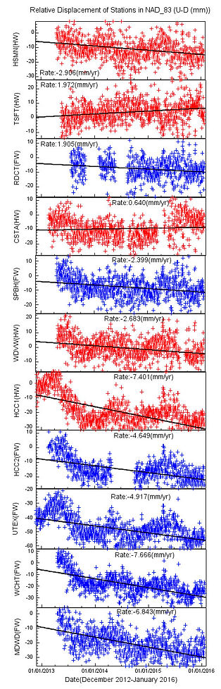
Figure.7. Three-component displacement time series of eleven GPS stations in NAD83 reference frame (left to right U-D, N-S and E-W) shows some seasonal signals in three directions.


Figure.8. Three-component displacement time series of eleven GPS stations reference to UTEX (left to right U-D, N-S and E-W).
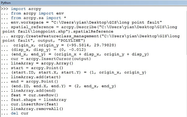
Figure.9. The Python script used to plot GPS velocity vectors. Create a feature first and then add the new row with the orirgin coordinates, displacement distance to construct geometry.
Groundwater data within the Long-Point Fault area was downloaded from USGS Groundwater Watch website (Fig.10.) (http://groundwaterwatch.usgs.gov/default.asp). Two real-time ground water data and 29 periodic data were used to examine the correlation between subsidence and groundwater-level change. The workflow of generating a groundwater head depth and level change equal value line is shown in (Fig.11.). First, import the data into ArcGIS to create a feature and then convert the feature into the DEM with Inverse Distance Weighted Interpolation (IDW) then with "Contour" tool to create contour and "Smooth" tool to smooth the line feature.


Figure.10. Groundwater data from USGS Groundwater watch website

Figure.11. Workflow to create the contour
LiDAR data is acuired from TLS scan in the field and is applied with Octree filter to reduce the data size and the terrain filter to get the bare-earth model. Once get the bare-earth model the data will be exported as ASCII file and LAS file which can be imported to ArcGIS to create a layer and with the interpolation to get the DEM while the interpolation the grid size needed to be defined since this study focus on the scault with scale to kilometer, the grid size is set to be 100x100m. This grid size may be too big for the resampling of the area with dense point clouds but for those area with less dense it would avoid aliasing to have it resample in a bigger size shile also maintain the feature we are interested. The interpolation used here is IDW since this study is dealing with the uneven distibuted points clouds (Fig.12.) and thus needs a more smooth interpolation although IDW can also give a smooth result it is more vulnerable to generate a "bull eye".

Figure.12. Bar-earth model of point clouds data of six TLS scans.